To see which steps in our algorithm yield zeros in the resulting parameter vector, we consider the inequality

$$ w \leq \lambda p w^{p-1}. $$

This inequality, and the curve bounding it

$$ w = \lambda p w^{p-1}, $$

defines the weight size w below which our gradient will step to zero (given that we truncate step sizes if they would overstep zero). Now, for every $\lambda$ there is a particular value of $p$ which maximizes the size of $w$. We can find the value of $p$ which maximizes this $w$ by considering the implicit partial derivative of $w$ with respect to $p$ given by

$$ \frac{\partial w(p, \lambda)}{\partial p} = \frac{\partial}{\partial p} \big( \lambda p w^{p-1} \big), $$

which we can algebraically manipulate into the following form:

$$ \frac{\partial w(p, \lambda)}{\partial p} = \frac{\partial}{\partial p} \Big( \lambda p \, e^{(p-1)\ln(w)} \Big). $$

This will more easily render the derivative by the steps below. First we use the chain rule,

$$ \frac{\partial w(p, \lambda)}{\partial p} = \lambda e^{(p-1)\ln(w)} + \Big( \frac{\partial w(p, \lambda)}{\partial p} \cdot \frac{1}{w} + \ln(w) \Big) \cdot \Big( \lambda p \, e^{(p-1)\ln(w)} \Big), $$

then by additional manipulation

$$ \frac{\partial w(p, \lambda)}{\partial p} = \lambda w^{p-1} + \frac{\partial w(p, \lambda)}{\partial p} \cdot \frac{1}{w} \cdot \lambda p w^{p-1} + \ln(w) \, \lambda p w^{p-1}, $$

$$ \frac{\partial w(p, \lambda)}{\partial p} \Big(1-\frac{1}{w} \lambda p w^{p-1}\Big) = \lambda w^{p-1} + \ln(w) \, \lambda p w^{p-1}, $$

finally yielding

$$ \frac{\partial w(p, \lambda)}{\partial p} = \frac{\lambda w^{p-1} + \ln(w) \, \lambda p w^{p-1}}{1-\frac{1}{W}\lambda p w^{p-1}}. $$

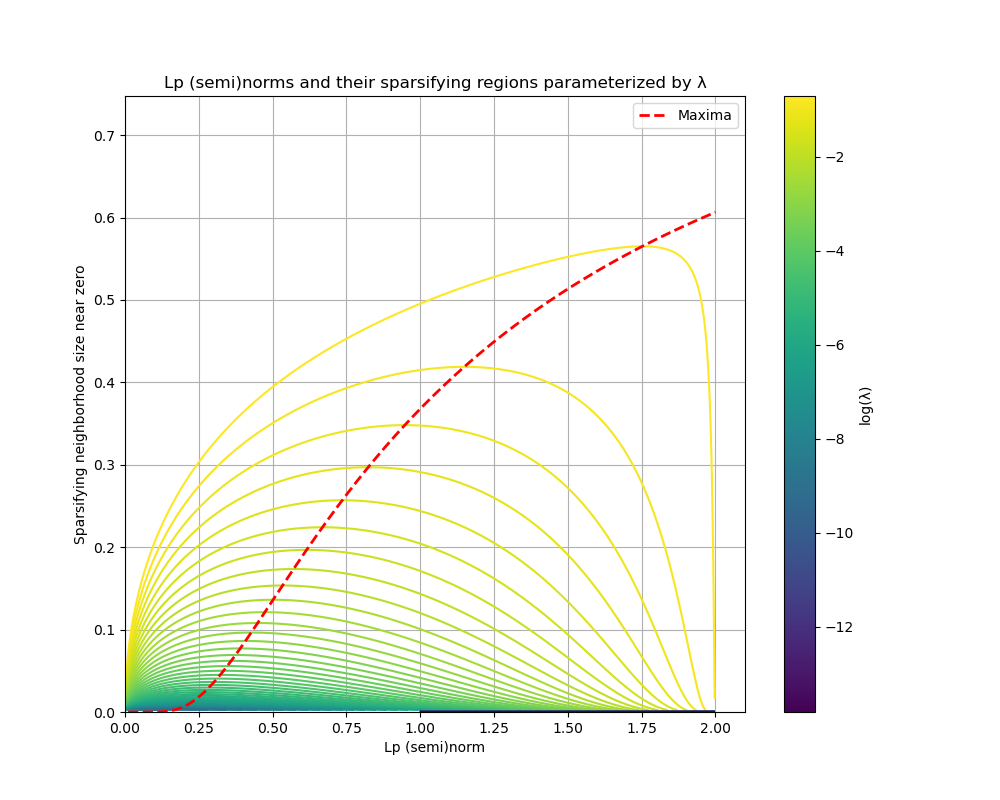
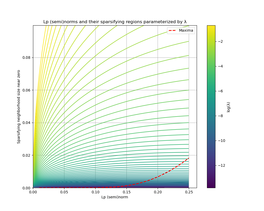
To find this derivative's ostensible maxima, we need to factor the numerator in the previous expression to get $\lambda w^{p-1}(1+p\ln(w))$. Since we are only concerned with values $0 < p \leq 2$ we need only consider when $0 = 1 + p \ln(w)$, which are (indeed) actual maxima in this range. This gives a relationship $w = e^{-1/p}$, but how do we relate this back to $\lambda$? If we insert this value back into the curve equation we can establish the relationship between $\lambda$ and the $p$ value at which our "sparsifying region" is maximized:

$$ e^{-1/p} = \lambda p \, e^{\frac{-1}{p}(p-1)}, $$

so that

$$ \frac{e^{-1/p}}{p \, e^{-\frac{1}{p}(p-1)}} = \frac{1}{p} e^{1-\frac{2}{p}} = \lambda. $$

As mentioned before, we are interested in the segment between $0 < p \leq 2$. This is important, as solving this equation requires the Lambert W function to yield

$$ p = \frac{-2}{W\ \left(\frac{- 2 \lambda}{e}\right)}. $$

In this case, this corresponds to a segment of the left branch of the Lambert W function; in other words we are specifically interested in

$$ p = \frac{-2}{W_{-1}\ \left(\frac{- 2 \lambda}{e}\right)}. $$

The relation above means that, given any particular $\lambda$, we can select an optimal target value $p$ which our annealing process can anneal towards. This value of $p$ represents a maximization of the region around 0 that will be stepped towards 0 at the next iteration. The behavior of these relations can be observed in the figures above.